40 Superior SQL Window Capabilities: A Full Information

On the planet of information science, SQL nonetheless stays the highly effective device for outlining the information, knowledge manipulation, knowledge aggregation and knowledge evaluation.

Whereas fundamental SQL instructions are very elementary, and everybody is aware of about it. If you wish to be the distinctive within the crowd then you must know superior options like window features that may unlock a number of capabilities for complicated knowledge transformations and insights. On this article, you’ll find out about these superior SQL window features that you simply concentrate on and how one can use them in your undertaking.

Distinction between Window Capabilities and Common Mixture Capabilities

Common mixture features like (SUM(), AVG(), COUNT() with out OVER()): These features collapse rows into abstract. It takes a gaggle of rows and return a single abstract row. For instance: “SELECT SUM(gross sales) FROM orders provides you complete variety of gross sales quantity.

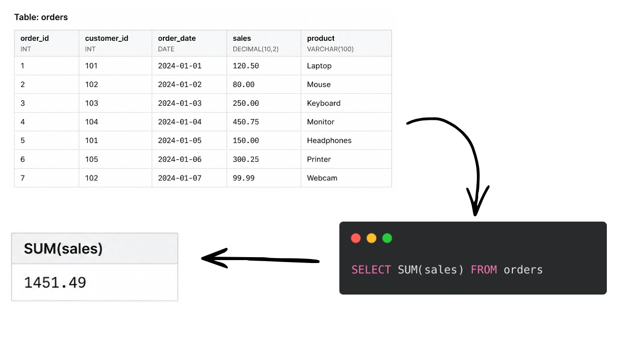
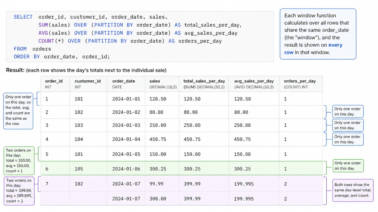
Home windows Capabilities like (SUM(), AVG(), COUNT() with OVER()): These features additionally carry out calculations on group of rows, however they return a consequence for each single row in your unique knowledge. This implies you may see the overall gross sales for the day subsequent to every particular person gross sales that occurred on that day.

The Magic OVER() Clause: Defining your window

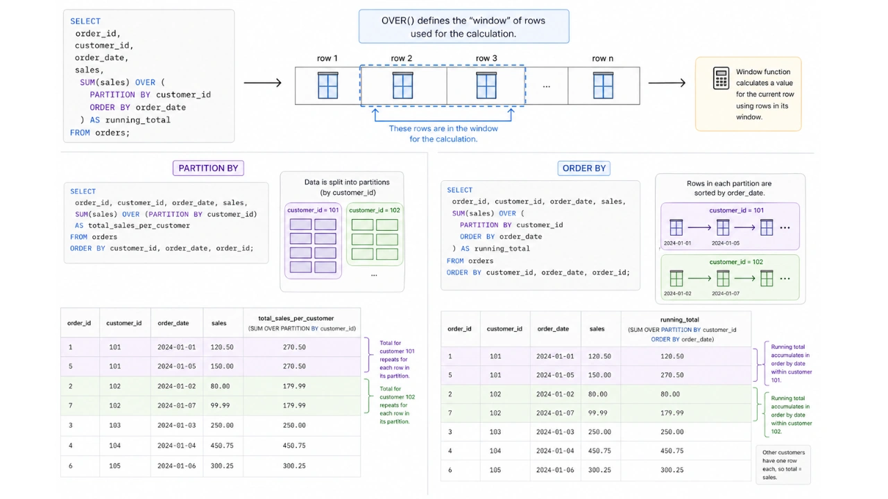
The OVER() clause is the center of each window perform. It tells SQL precisely which rows to incorporate in your window for the calculation. Inside OVER(), you need to use a couple of necessary key phrases:

• PARTITION BY: That is like saying “Group my knowledge by this column”. For instance, PARTITION BY customer_id means window perform will restart its calculation for every new buyer.
• ORDER BY: This tells SQL how one can type the rows with in every group(or the entire dataset if there’s no PARTITION BY). That is tremendous necessary for features that care about sequence, like discovering the primary or subsequent merchandise.

Understanding Window Frames: ROWS vs RANGE vs GROUPS

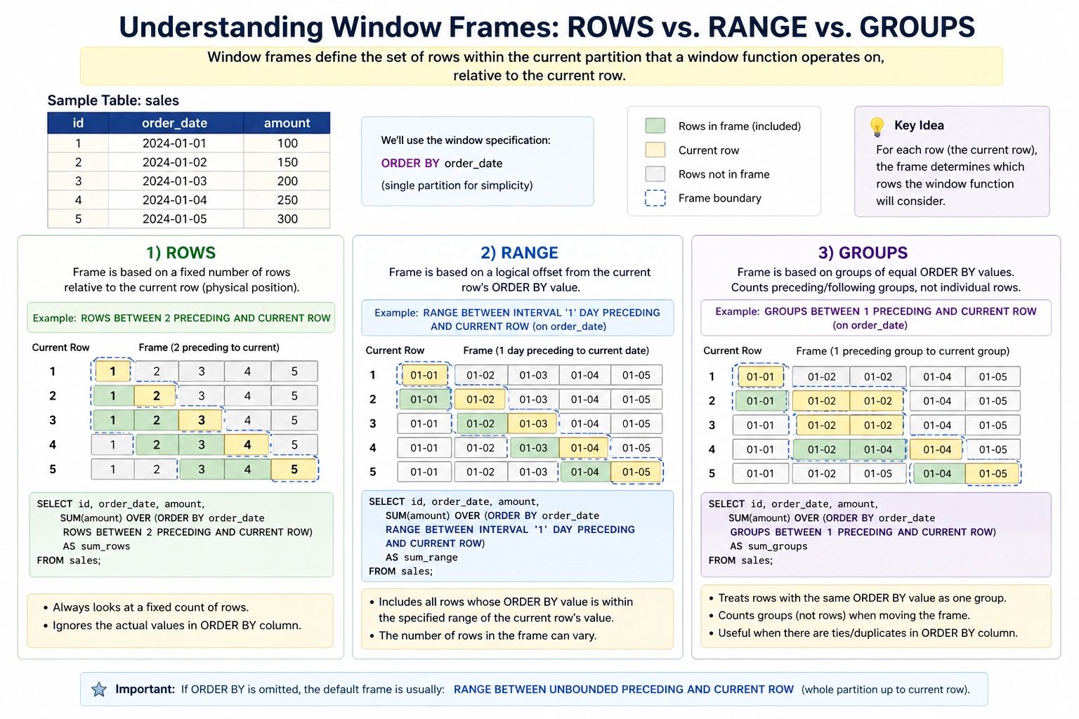
Window frames specify the subset of rows throughout the present partition that the window perform ought to function on. They’re outlined relative to the present row and are essential for calculations like transferring averages or cumulative sums.

• ROWS: Defines the body based mostly on a hard and fast variety of rows previous or following the present row. For instance, ROWS BETWEEN 2 PRECEDING AND CURRENT ROW consists of the present row and the 2 previous rows.
• RANGE: Defines the body based mostly on a logical offset from the present row’s worth within the ORDER BY clause. As an example, RANGE BETWEEN 100 PRECEDING AND CURRENT ROW would come with all rows whose ORDER BY worth is inside 100 models of the present row’s worth.
• GROUPS: (Much less widespread, however obtainable in some superior SQL dialects like Oracle) Defines the body based mostly on a logical group of rows, much like RANGE however typically used with extra complicated grouping logic.

The Important Rating and Numbering Capabilities

These features are good for sorting your knowledge and assigning ranks or numbers inside teams. They assist you rapidly discover the most effective, worst or just depend gadgets in a sequence.

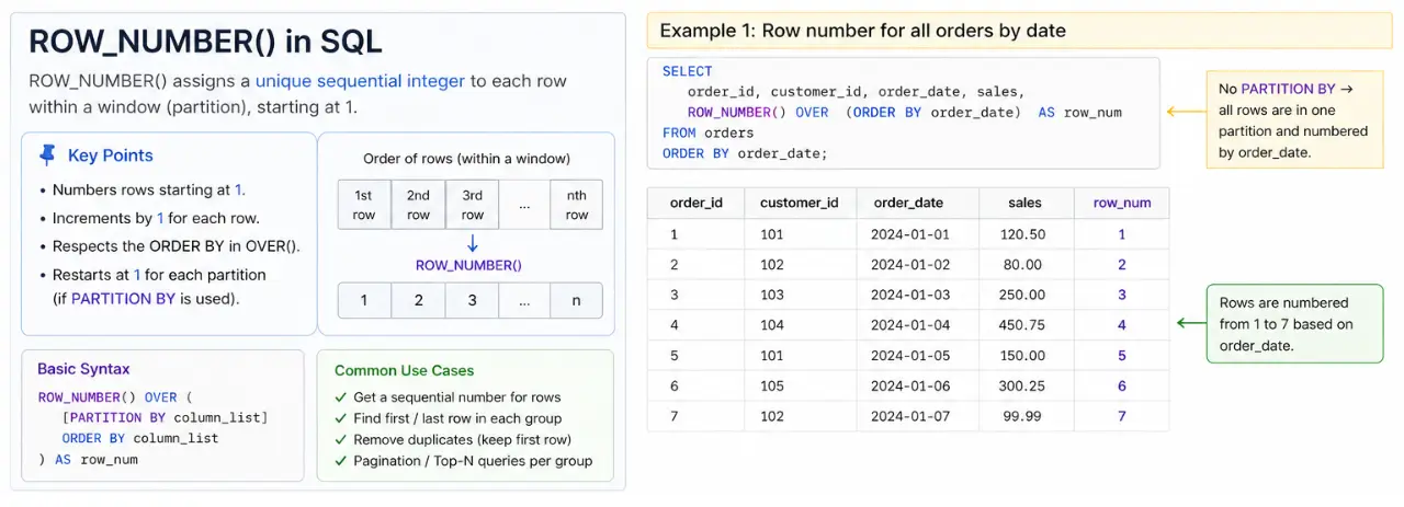
ROW_NUMBER(): Giving Every Row a Distinctive Quantity

ROW_NUMBER() assigns a novel, sequential quantity(ranging from 1) to every row inside group. It’s excellent whenever you want a easy, distinct ID for every merchandise based mostly on a selected order.

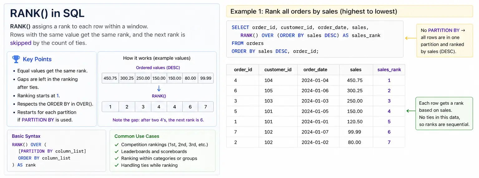
RANK(): Rating with Gaps for Ties

RANK() provides rank to every row inside its group. If two rows have the identical worth(a “tie”), they get the identical rank. The following ranks then “skips” numbers. So if two gadgets are ranked #1, the subsequent merchandise can be #3(skipping #2)

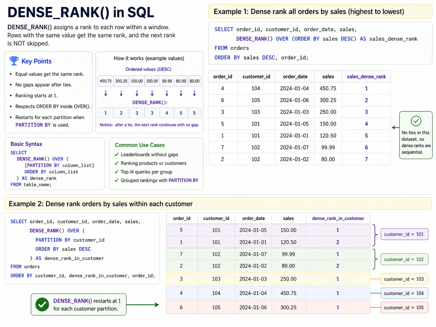
DENSE_RANK(): Rating With out Gaps

DENSE_RANK() is similar to RANK() nevertheless it doesn’t skip numbers the place there are ties. If two gadgets are ranked #1, the subsequent merchandise will probably be #2(no skipped numbers)

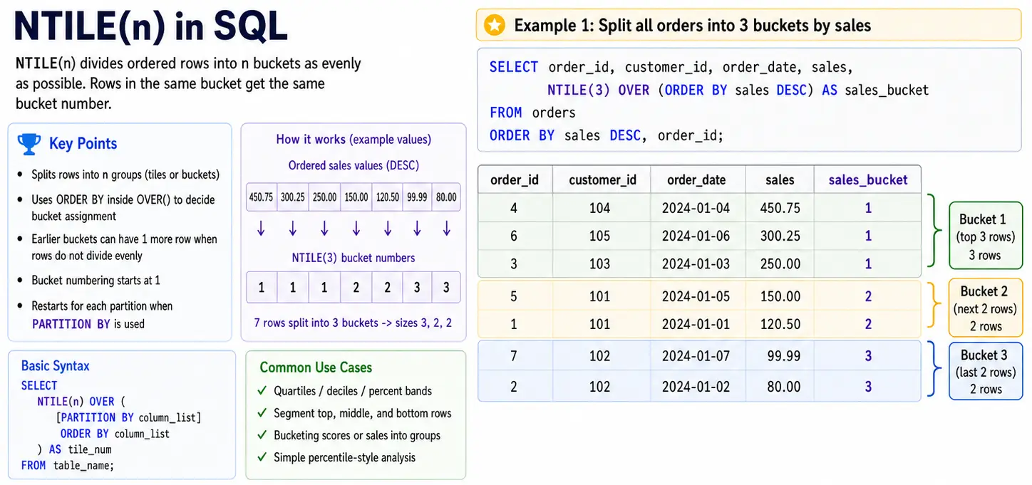
NTILE(n): Dividing into Equal Teams

NTILE(n) divides your rows into “n” equal teams(for equal as attainable). It assigns a quantity from 1 o ‘n’ to every group. That is nice for creating segments like quartiles(4 teams), deciles(10 teams) or another bucket for evaluation.

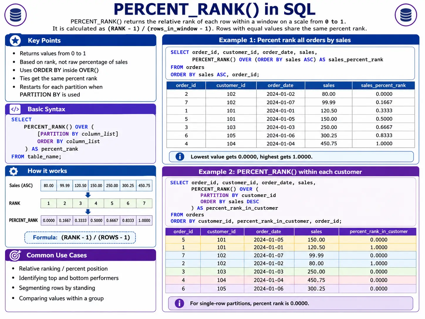
PERCENT_RANK(): Displaying Relative Place

PERCENT_RANK() let you know the relative rank of a row inside its group as a proportion from 0 to 1. It reveals you the place a selected merchandise stands in comparison with all others in its group.
The Important Rating and Numbering Capabilities.

Navigation & Positional Capabilities

These features are like time travellers on your knowledge! They allow you to take a look at values from rows earlier than or after the present inside your window. That is tremendous helpful for evaluating issues over time, like seeing how at the moment’s gross sales examine to yesterday’s.

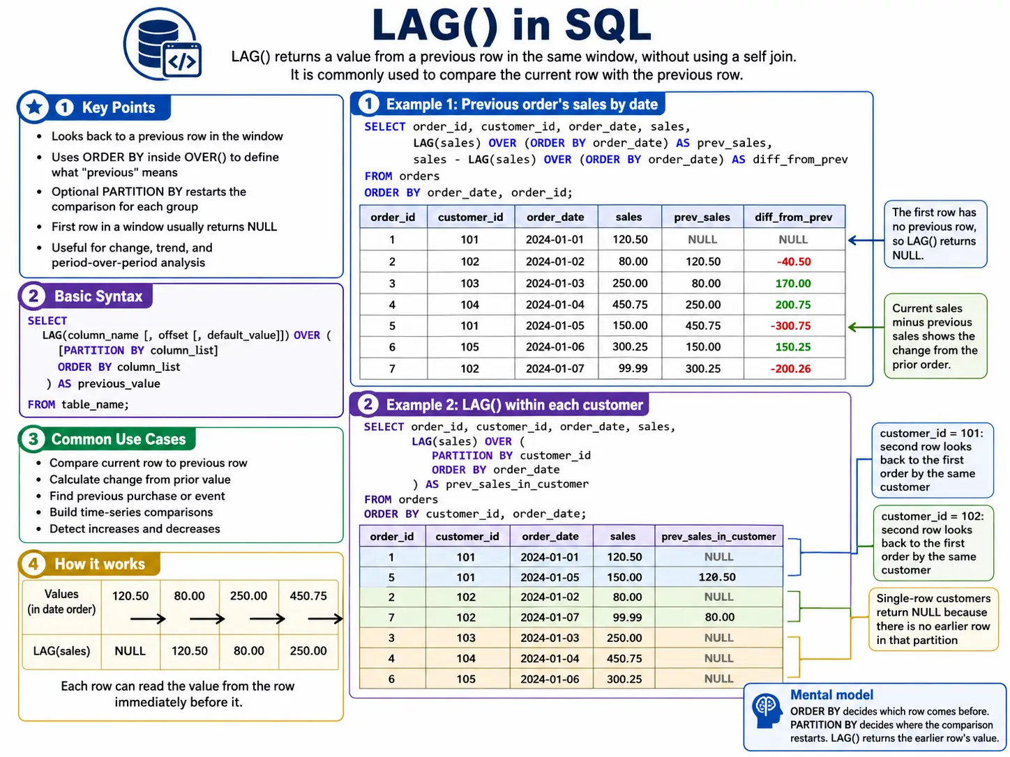
LAG(): Trying Again in Time

LAG() enables you to seize a worth from a row that got here earlier than the present row. You’ll be able to specify what number of rows again you need to look. It’s excellent for calculating issues like “change from earlier day” or “final identified worth”

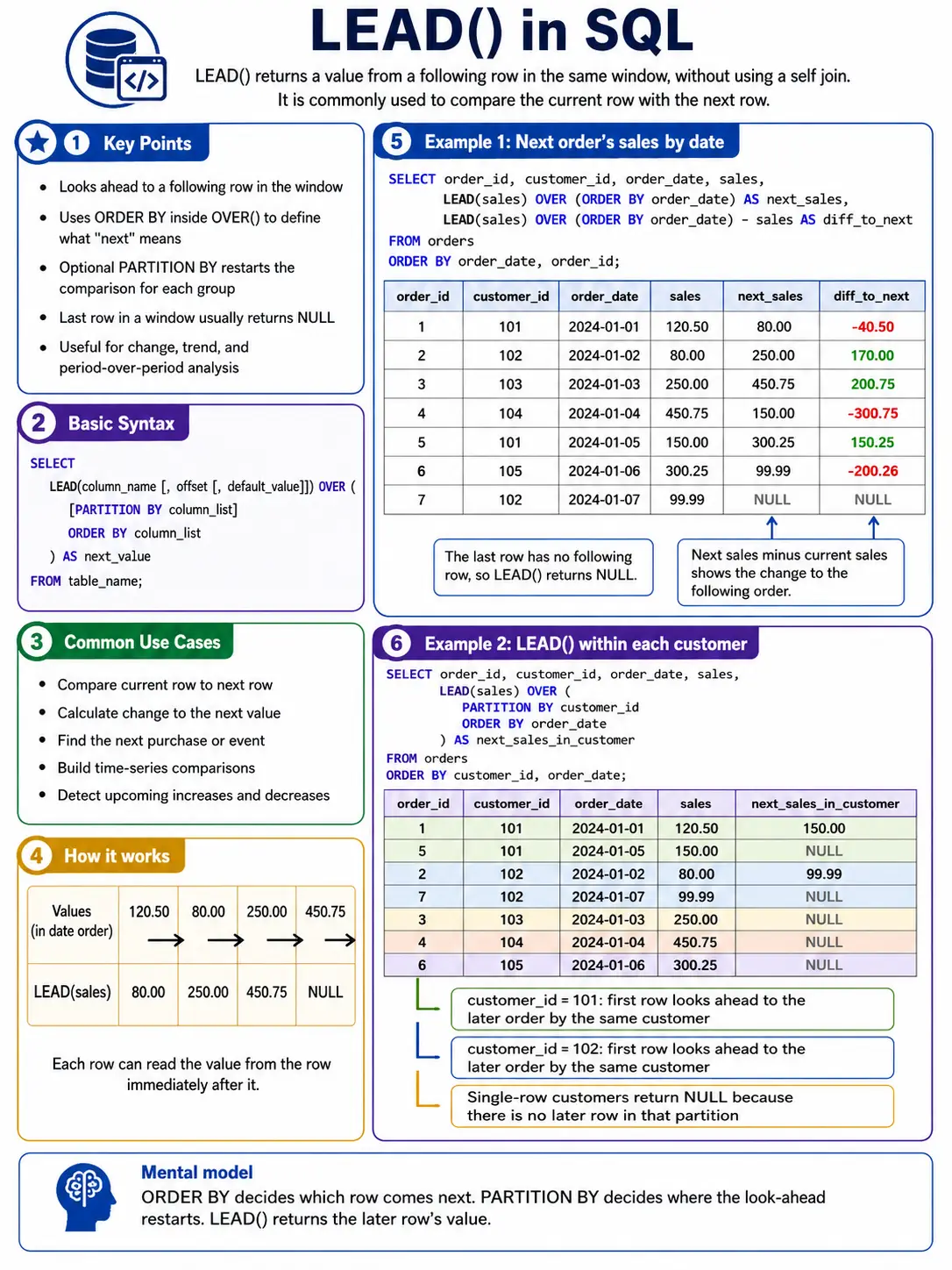
LEAD(): Peeking into the Future

LEAD() is the alternative of LAG(). It enables you to seize a worth from a row that comes after the present row. That is nice for evaluating to future values, like “subsequent month’s forecast” or “the occasion in a sequence”

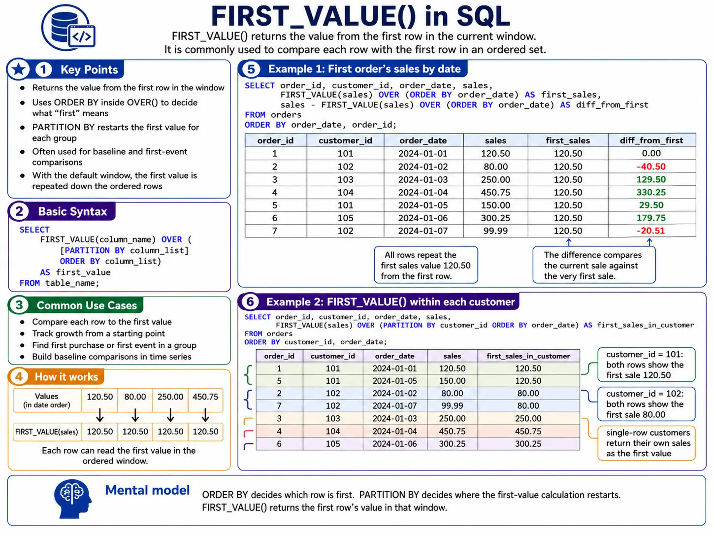
FIRST_VALUE(): Discovering the beginning of the Group

FIRST_VALUE() merely returns the worth from the very first row in your present window. That is helpful for setting a baseline or evaluating every part to the preliminary state.

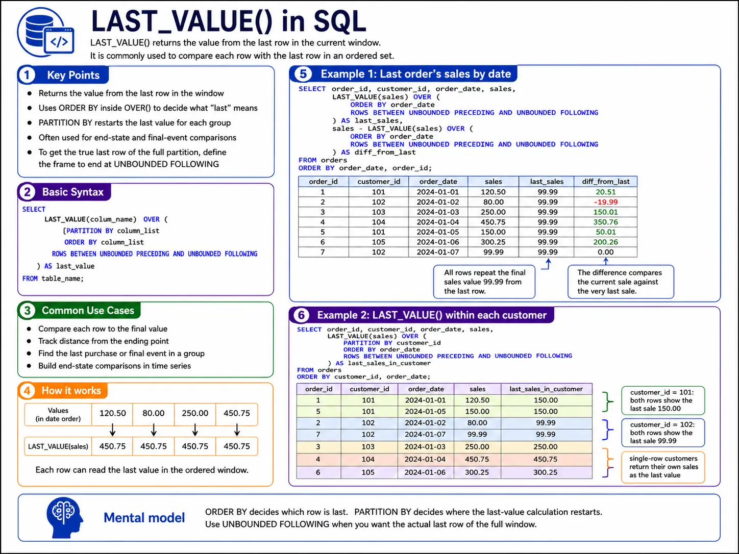
LAST_VALUE(): Discovering the Finish of the Group

LAST_VALUE() returns the worth from the final row in your present window. Watch out with this one! By default, the window typically solely appears as much as the present row. To actually get the ‘final worth of the complete group‘, you normally must explicitly inform SQL to take a look at all rows within the partition utilizing a particular body definition like ‘ROWS BETWEEN UNBOUNDED PRECEDING AND UNBOUNDED FOLLOWING’.

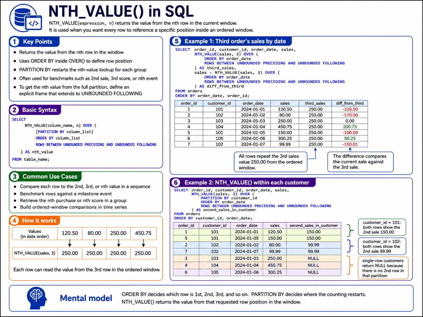
NTH VALUE(expression, n): Selecting a selected Row

NTH_VALUE() is extra versatile model of FIRST_VALUE() and LAST_VALUE(). It enables you to decide the worth from the ‘n^th row in your window. So, you possibly can get the 2nd, third, or any particular row’s worth.

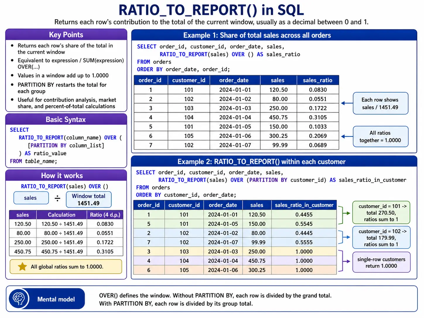
RATIO_TO_REPORT(): Used Particularly in Oracle/BigQuery

RATIO_TO_REPORT() tells you what proportion a selected worth contributes to the overall sum of its group. It’s nice for understanding proportions.

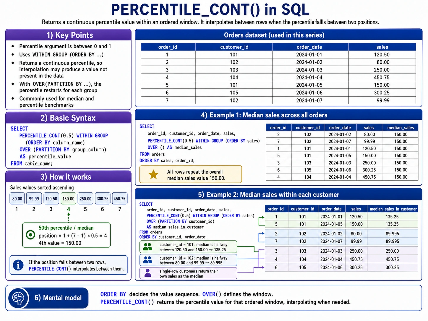
PERCENTILE_CONT(): Discovering the Center Floor

PERCENTILE_CONT() helps you discover a percentile (just like the median, which is the fiftieth percentile) in a method that can provide you a worth between precise knowledge factors. It’s like drawing a clean curve by way of your knowledge to seek out the precise level.

Superior Statistical & Regression Capabilities

These features deliver severe arithmetic energy straight into your SQL Queries. They assist knowledge scientists to dig deeper into knowledge patterns, measure how unfold out knowledge is, and even to seek out relationships between completely different columns.

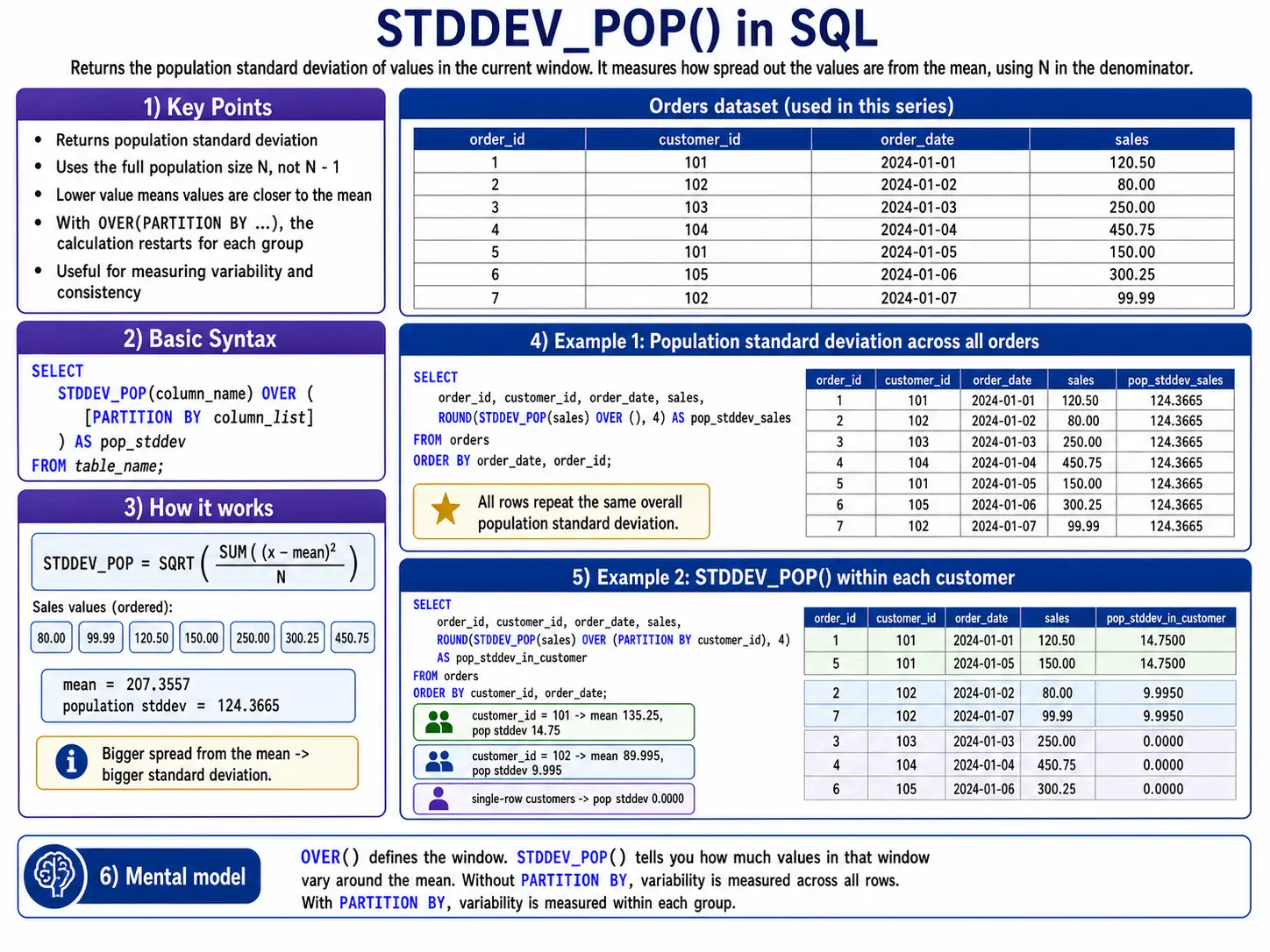
STDDEV_POP(): How Unfold Out is My Entire Knowledge?

STDDEV_POP() calculates the usual deviation for a whole group of information (the “inhabitants”). It tells you, on common, how far every knowledge level is from the typical of the group. A small quantity means knowledge factors are near the typical; a big quantity means they’re extra unfold out.

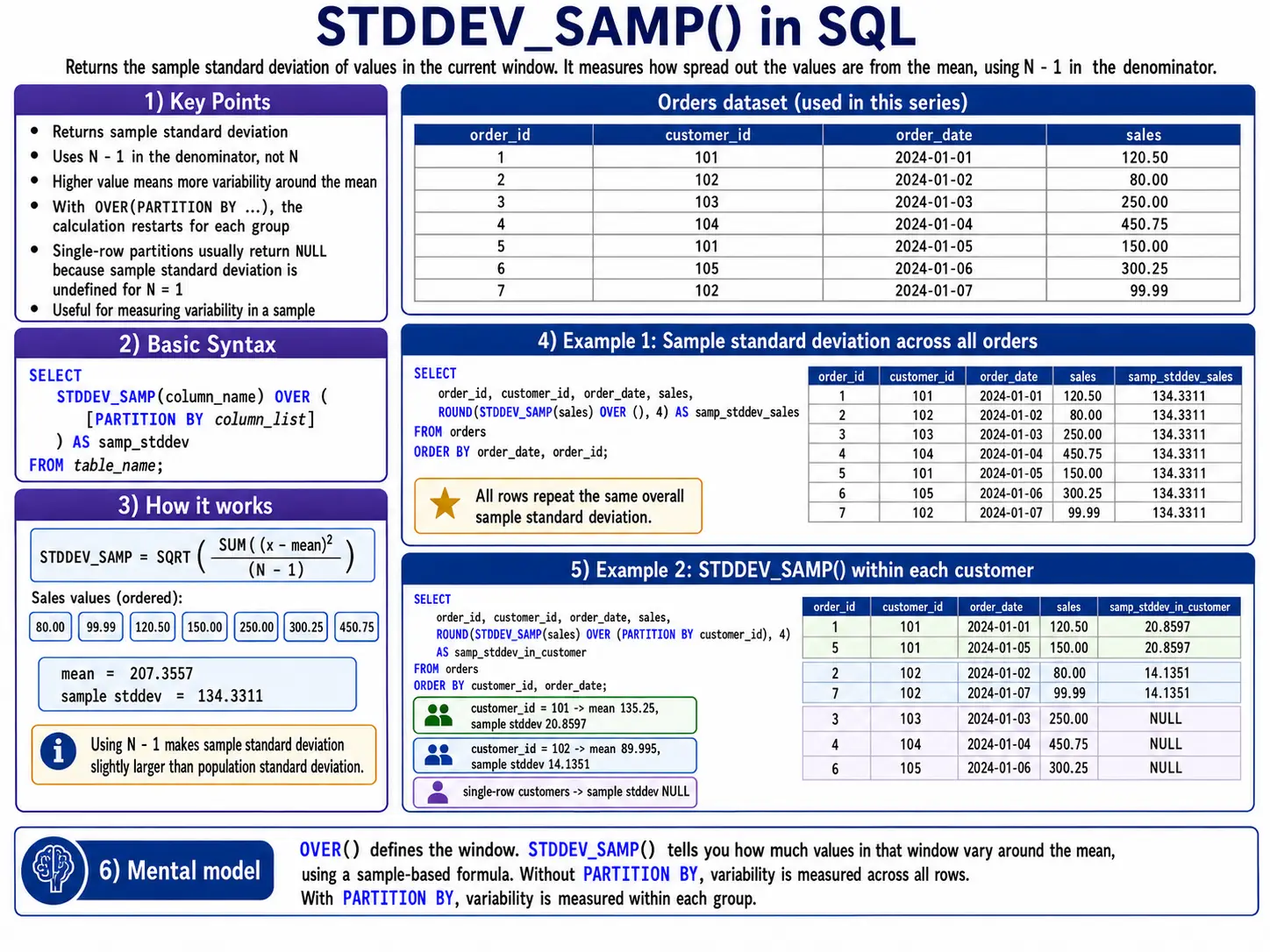
STDDEV_SAMP(): How Unfold Out is my Pattern Knowledge?

STDDEV_SAMP() is much like STDDEV_POP(), nevertheless it’s used when your knowledge is only a pattern of a bigger group. It makes a slight adjustment to present a greater estimate of the usual deviation of the total inhabitants.

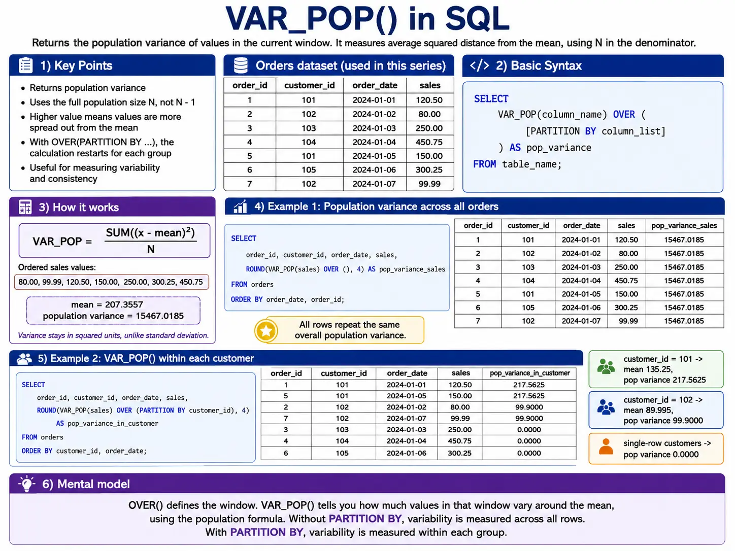
VAR_POP(): The Sq. of Unfold

VAR_POP() calculates the variance for a whole group. Variance is just the usual deviation squared. It’s one other solution to measure how unfold out your knowledge is.

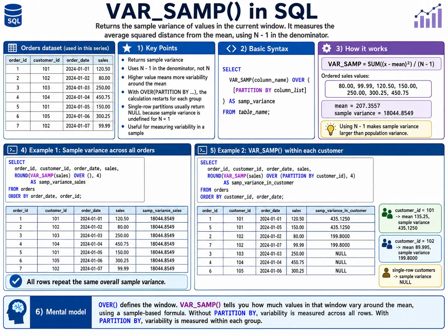
VAR_SAMP(): Pattern Variance

Like STDDEV_SAMP(), this calculates the variance whenever you solely have a pattern of the information. For Instance: Estimate the variance in product weights from a high quality management pattern.

SELECT
    batch_id,
    product_weight,
    VAR_SAMP(product_weight) OVER (PARTITION BY batch_id) AS sample_weight_variance
FROM
    quality_control;

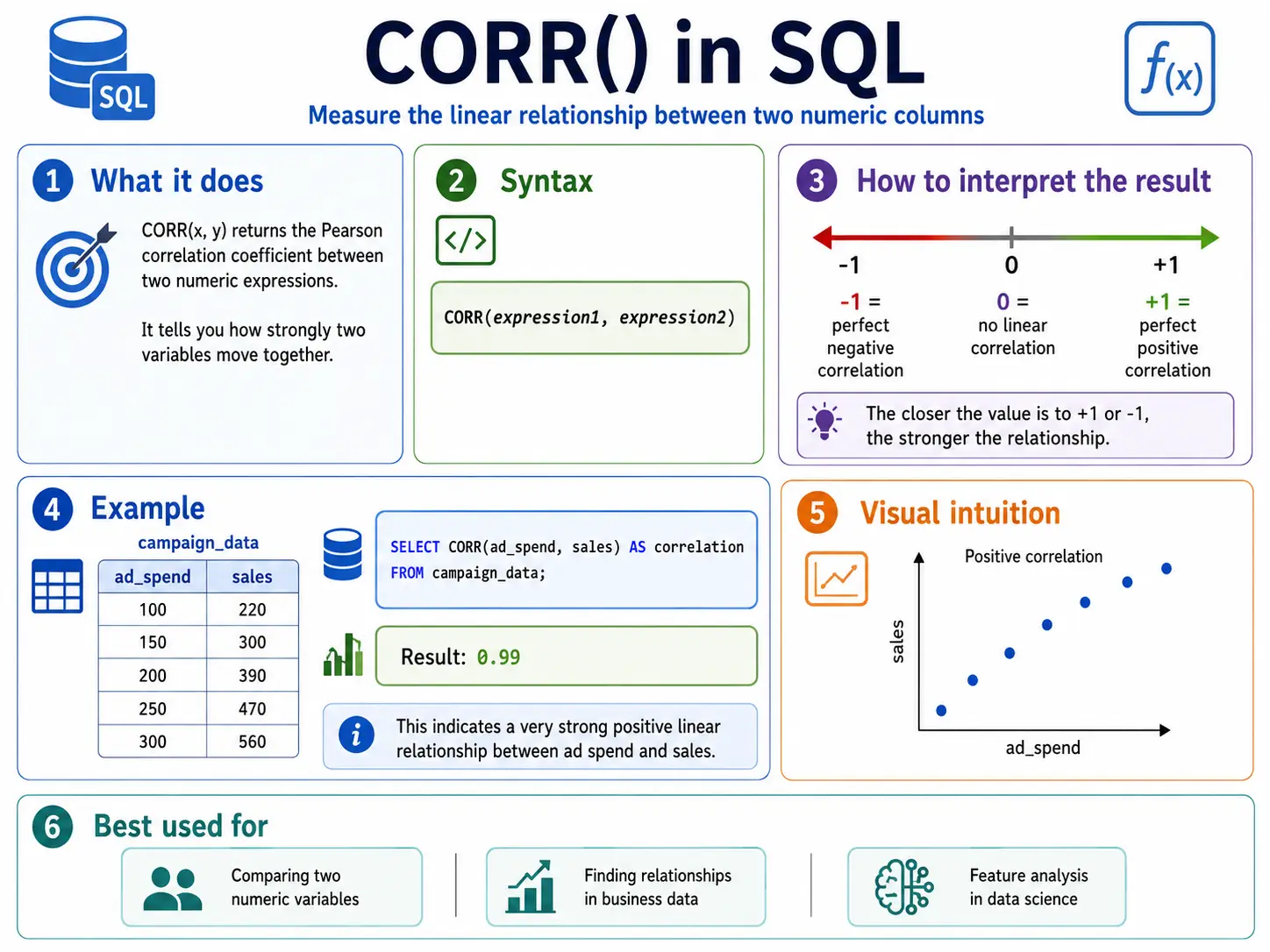
CORR(): Discovering Relationships (Correlation)

CORR() measures how strongly two issues are associated. It provides a quantity between -1 and 1. A quantity near 1 mens as one goes up, the opposite goes up. Near -1 means as one goes up, the opposite goes down. Near 0 means no actual relationship.

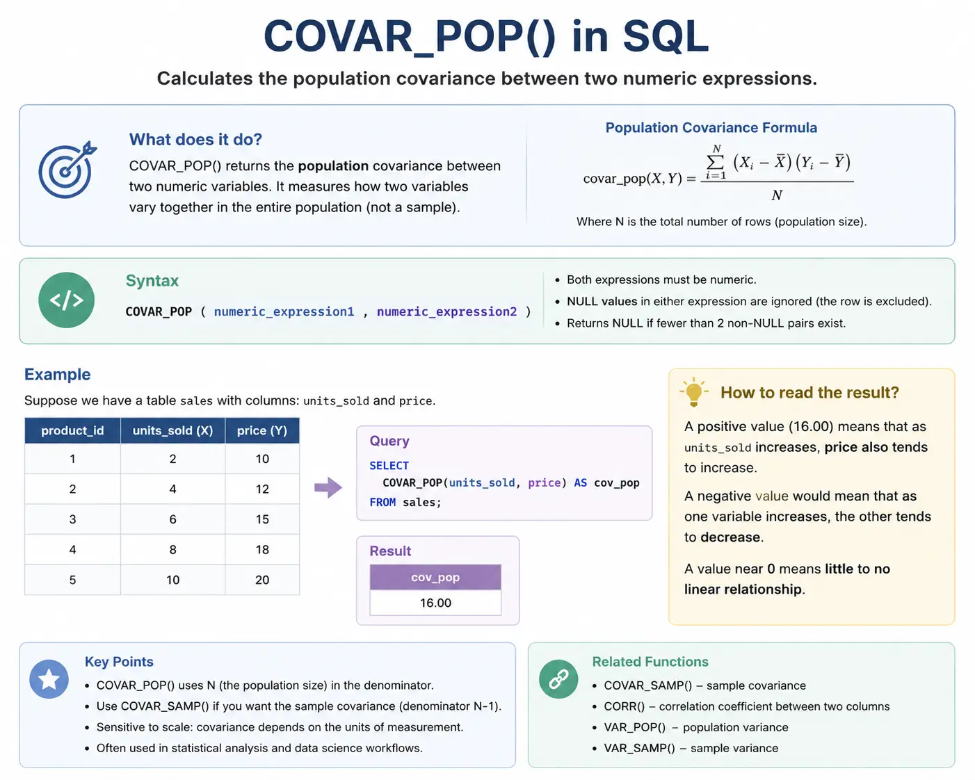
COVAR_POP(): How Issues Transfer Collectively (Covariance)

COVAR_POP() measures covariance, which is analogous to correlation however not scaled between -1 and 1. It tells you the path of the connection (optimistic or detrimental) between two variables for the entire inhabitants.

COVAR_SAMP(): Pattern Covariance

That is the pattern model of covariance, used whenever you don’t have all the information.

Instance: Estimate the covariance between web site load time and bounce price based mostly on a pattern of consumer periods.

SELECT
    session_id,
    load_time_ms,
    bounce_flag,
    COVAR_SAMP(load_time_ms, bounce_flag) OVER () AS sample_covariance
FROM
    session_sample;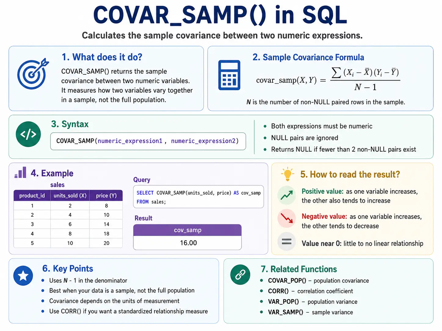

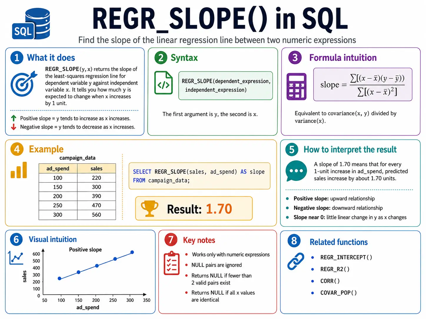
REGR_SLOPE(): Drawing a Pattern Line (Slope)

Think about drawing a “finest match” line by way of a scatter plot of your knowledge. REGR_SLOPE() tells you the steepness (slope) of that line. It helps you see the overall development.

REGR_INTERCEPT(): The place the Pattern Line Begins

REGR_INTERCEPT() tells you the place that “finest match” development line crosses the start line (the y-axis).

Instance: If we undertaking our gross sales development backward to month zero, what would the beginning gross sales be?

SELECT
    month_number,
    gross sales,
    REGR_INTERCEPT(gross sales, month_number) OVER () AS baseline_sales_estimate
FROM
    monthly_sales;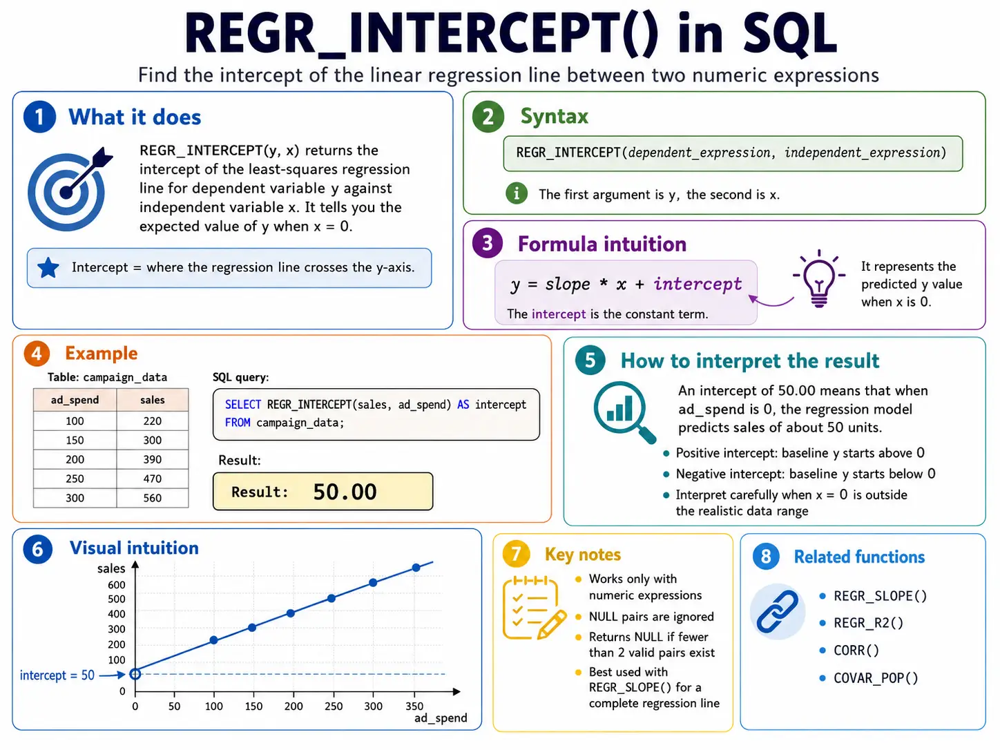

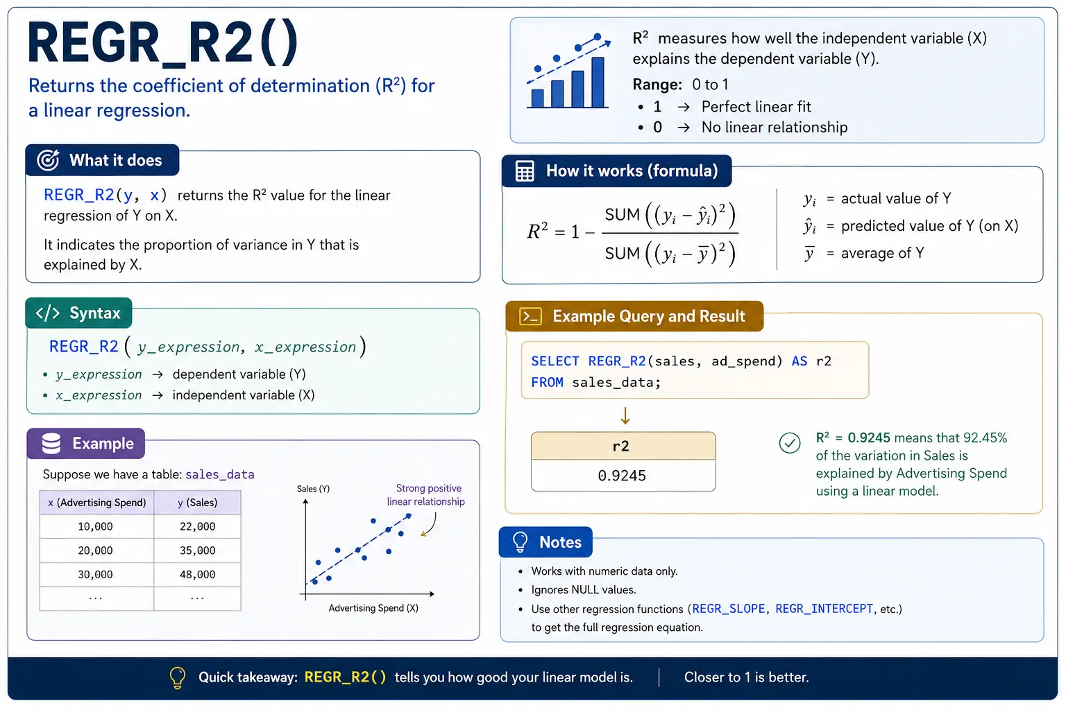
REGR_R2(): How Good is the Pattern Line?

REGR_R2() (R-squared) tells you ways properly your development line truly matches the information. A rating near 1 means the road is an excellent match; near 0 means the road doesn’t clarify the information properly in any respect.

Distribution & Likelihood Capabilities

These features assist you perceive the form of your knowledge. They let you know the place a selected worth sits in comparison with every part else, or assist you discover values at particular factors within the distribution.

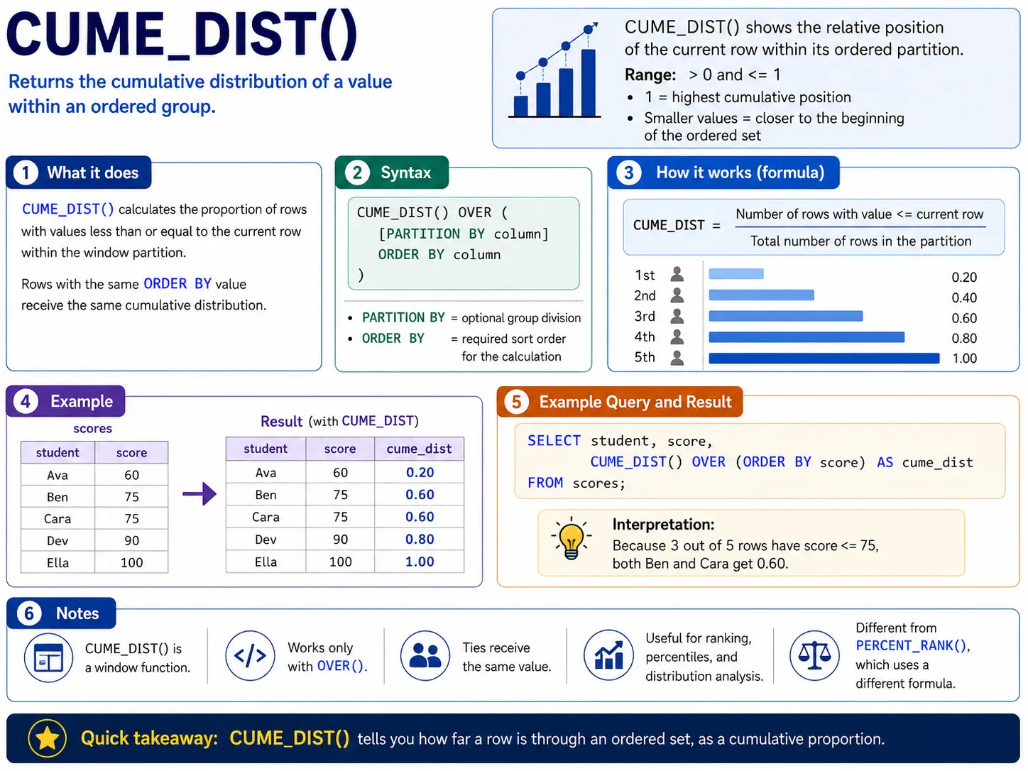
CUME_DIST(): The place Does This Row Stand?

CUME_DIST() tells you what fraction of the rows have a worth lower than or equal to the present row’s worth. It’s like asking, “What proportion of individuals scored the identical or decrease than me?” The result’s a quantity between 0 and 1.

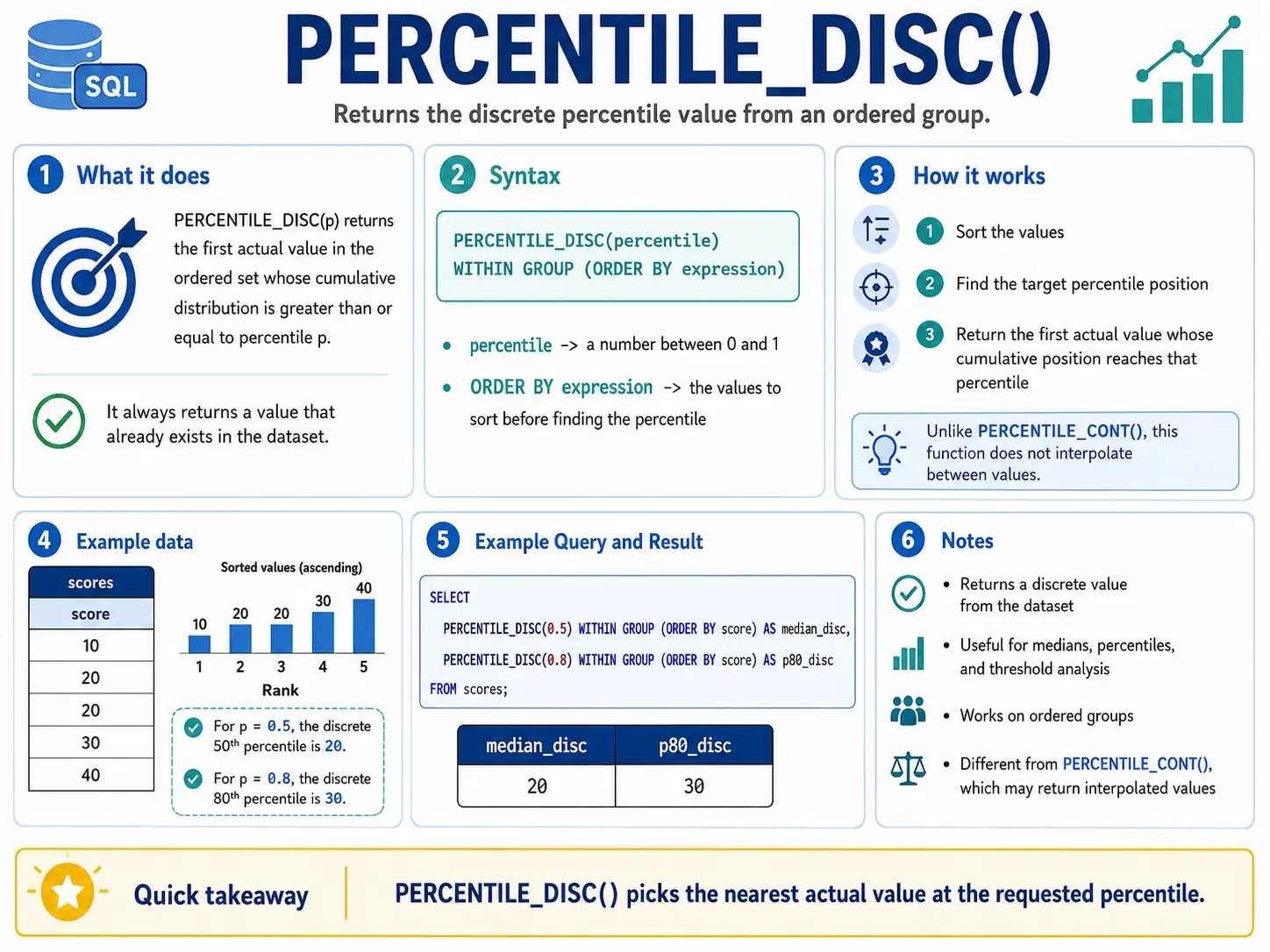
PERCENTILE_DISC(): Discovering an Precise Percentile Worth

PERCENTILE_DISC() helps you discover a particular worth out of your knowledge that represents a sure percentile (just like the fiftieth percentile for the median). The secret is that it’ll solely return an precise worth that exists in your knowledge, it received’t invent a brand new one. It finds the primary worth whose cumulative distribution is bigger than or equal to the percentile you ask for

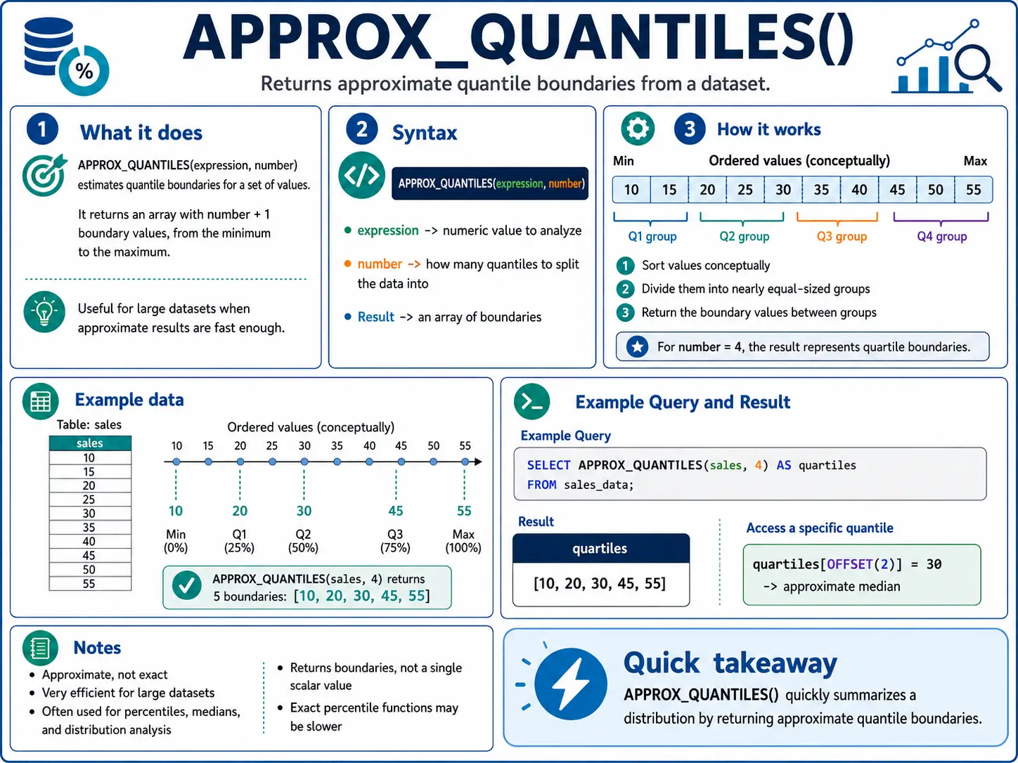
APPROX_QUANTILES(): (BigQuery) Quick Percentiles for Large Knowledge

When you’ve got large quantities of information, calculating actual percentiles might be very gradual. APPROX_QUANTILES() provides you a really shut estimate a lot quicker. You inform it what number of buckets you need (e.g., 100 for percentiles), and it returns an array of these approximate quantile values.

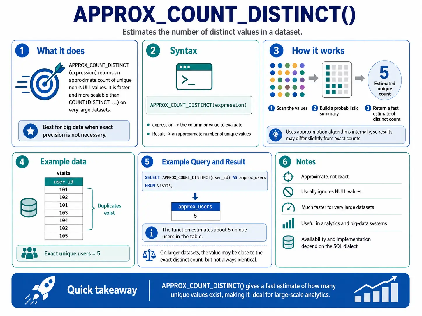
APPROX_COUNT_DISTINCT(): Quick Distinctive Counts

Just like APPROX_QUANTILES(), this perform provides you a quick estimate of what number of distinctive gadgets are in an enormous dataset. It’s a lot faster than COUNT(DISTINCT ...) when exactness isn’t essential, however pace is.

Mixture Capabilities as Home windows

You already know these features (SUM, AVG, COUNT, MIN, MAX) from fundamental SQL. However whenever you add the OVER() clause, they turn into tremendous highly effective for calculating issues like operating totals and transferring averages with out squishing your knowledge into single abstract rows.

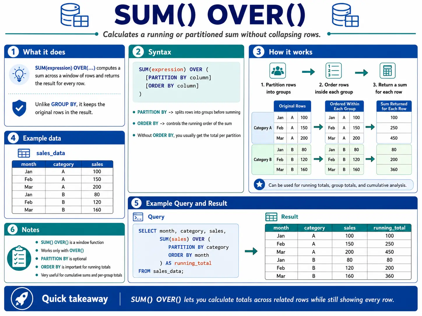
SUM() OVER(): The Working Complete

SUM() with OVER() and an ORDER BY clause creates a operating complete. This implies for every row, it provides up the present worth and all of the values earlier than it in that group. It’s excellent for seeing how a complete grows over time.

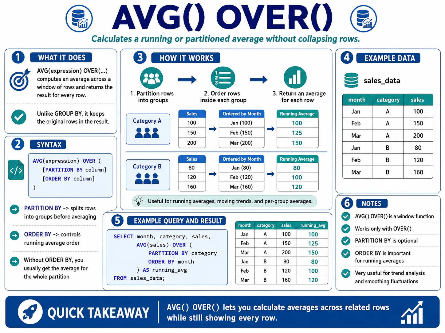
AVG() OVER(): The Shifting Common

AVG() with OVER() and a selected window body (like ROWS BETWEEN 6 PRECEDING AND CURRENT ROW) calculates a transferring common. That is tremendous helpful for smoothing out knowledge that jumps round loads (like each day web site visits) so you may see the actual developments extra clearly.

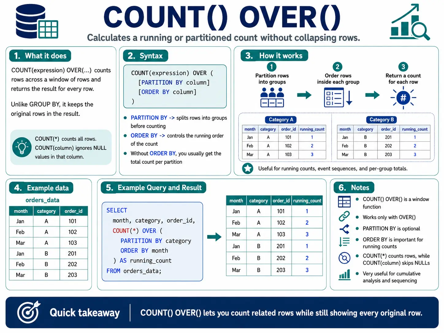
COUNT() OVER(): Counting Occasions in a Window

COUNT() with OVER() can provide you a operating depend of occasions or depend what number of gadgets fall inside a selected window. That is helpful for seeing what number of instances one thing has occurred as much as a sure level.

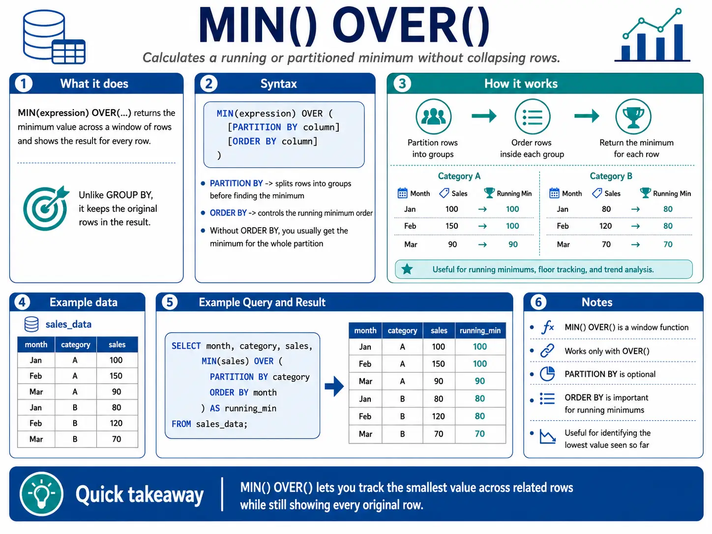
MIN() OVER(): Discovering the Lowest Level in a Window

MIN() with OVER() helps you discover the smallest worth inside a sliding window. That is helpful for monitoring minimums over a interval, just like the lowest inventory value within the final month.

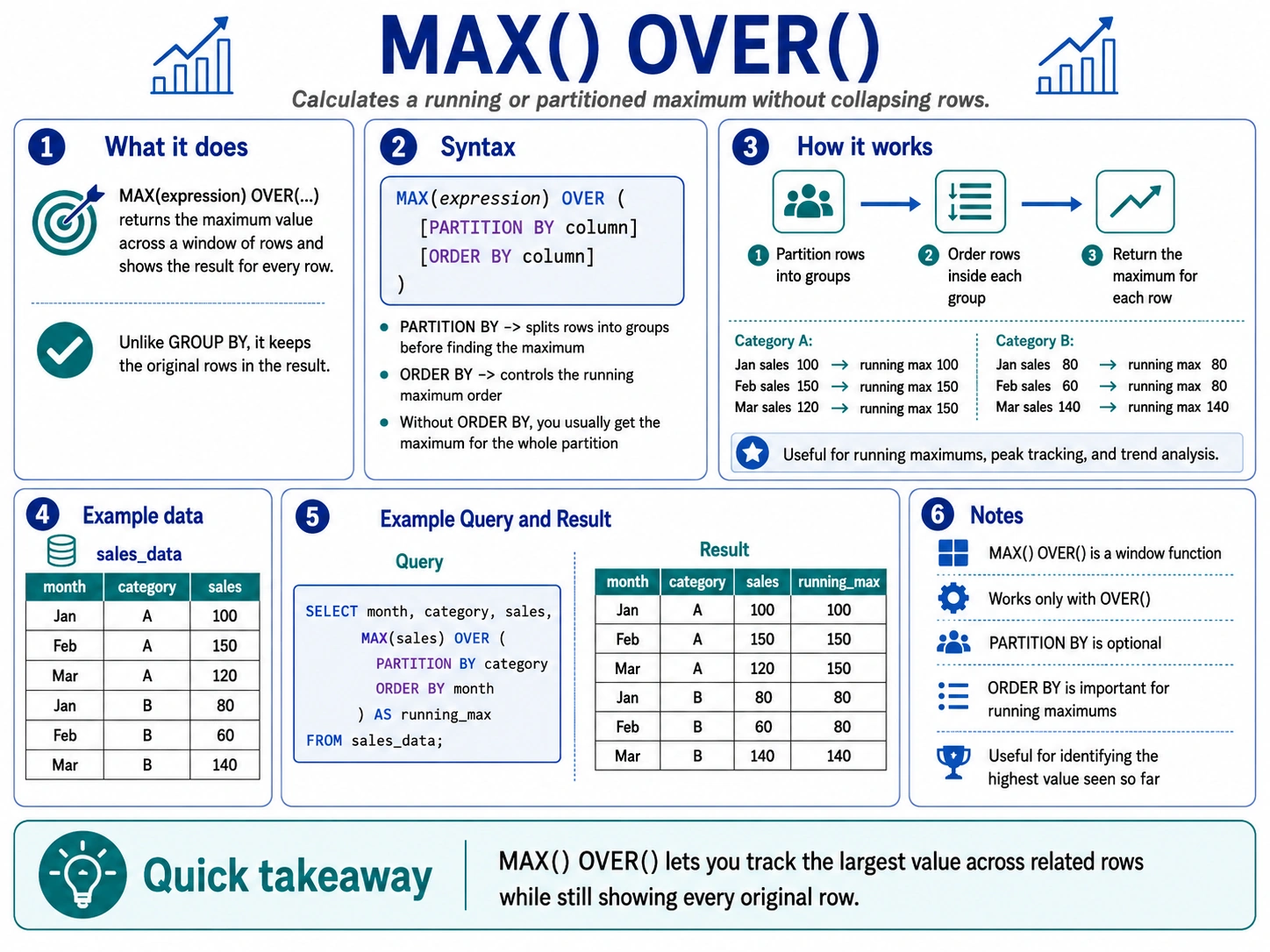
MAX() OVER(): Discovering the Highest Level in a Window

Equally, MAX() with OVER() finds the most important worth inside a sliding window. That is nice for monitoring peaks, like the very best temperature recorded within the final 24 hours.

Specialised Analytic & Platforms Particular Capabilities

Past the widespread features, many fashionable databases provide distinctive window features which are tremendous highly effective for particular duties. These may be a bit completely different relying on whether or not you’re utilizing BigQuery, Snowflake, Oracle, or PostgreSQL, however all of them assist you do extra superior knowledge science.

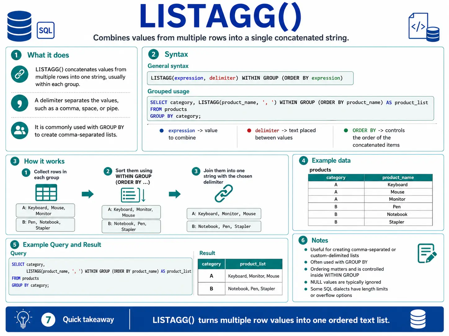
LISTAGG(): (Oracle/Snowflake) Gathering Textual content into One String

LISTAGG() takes values from many rows and squishes them right into a single string, separated by one thing you select (like a comma). It’s nice for making lists of things associated to a gaggle.

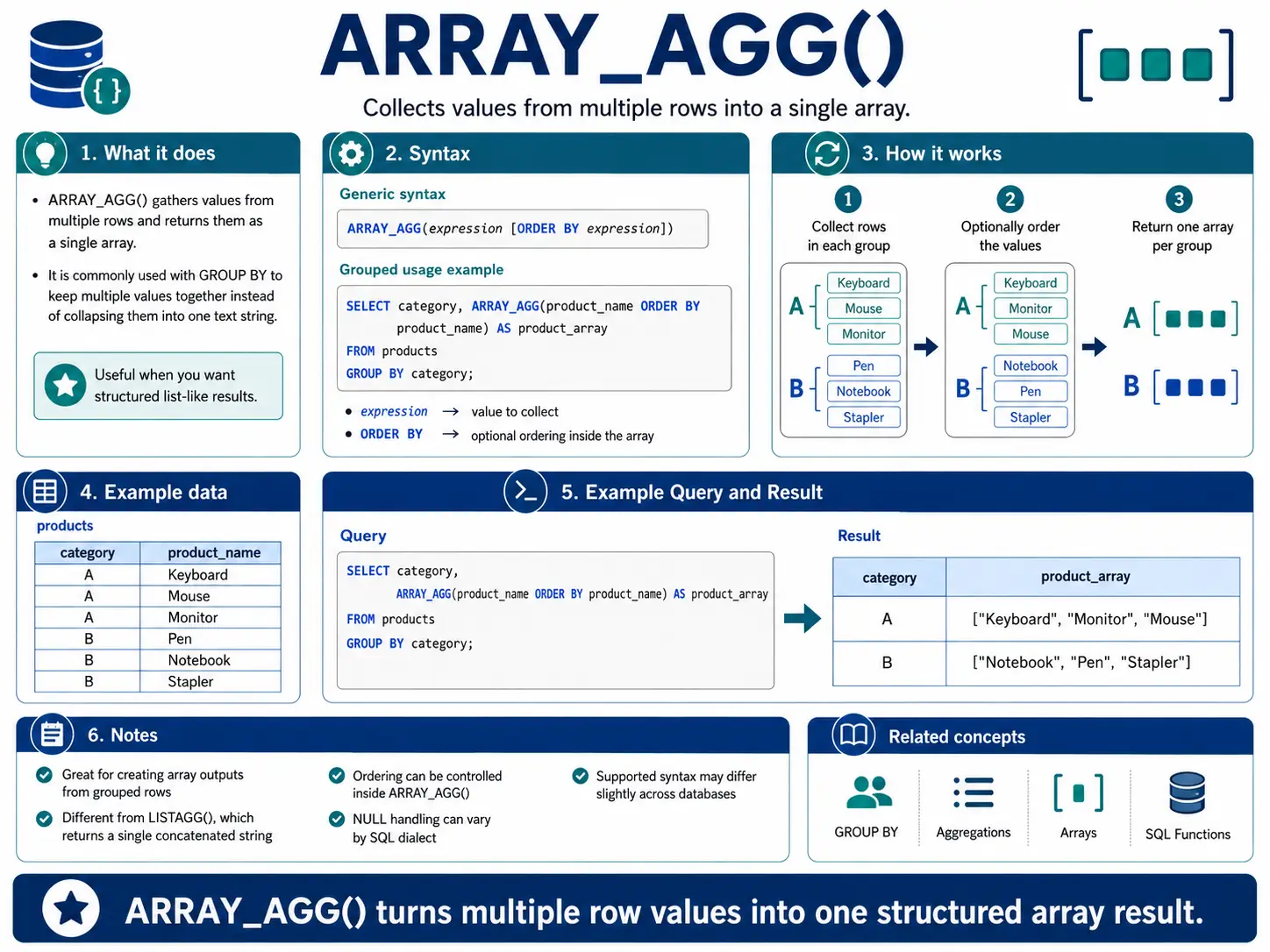
ARRAY_AGG(): (BigQuery/PostgreSQL) Gathering Objects right into a Record (Array)

ARRAY_AGG() is much like LISTAGG(), however as an alternative of a single string, it collects values into an array (a structured listing). That is very helpful in databases that deal with complicated knowledge varieties, letting you retain associated gadgets collectively.

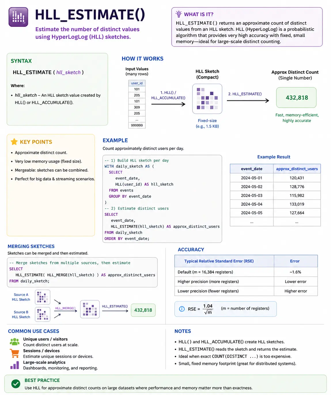
HLL_ESTIMATE(): (Snowflake) Shortly Counting Distinctive Issues in Large Knowledge

HLL_ESTIMATE() makes use of a intelligent trick (referred to as HyperLogLog) to rapidly estimate what number of distinctive gadgets are in a really massive dataset. When counting actual distinctive gadgets is just too gradual, this perform provides you a good-enough reply very quick.

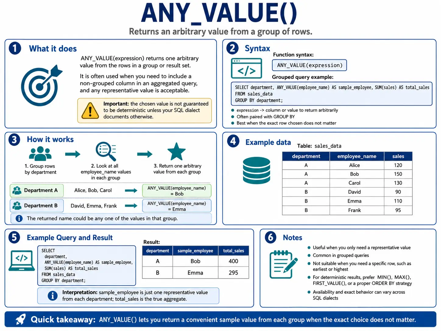
ANY_VALUE(): (BigQuery) Simply Seize Any Worth

ANY_VALUE() is an easy perform that returns any worth from a gaggle. It’s helpful whenever you don’t care which particular worth you get, simply that you simply get one from that group. This helps keep away from errors when that you must embrace a non-grouped column in your outcomes.

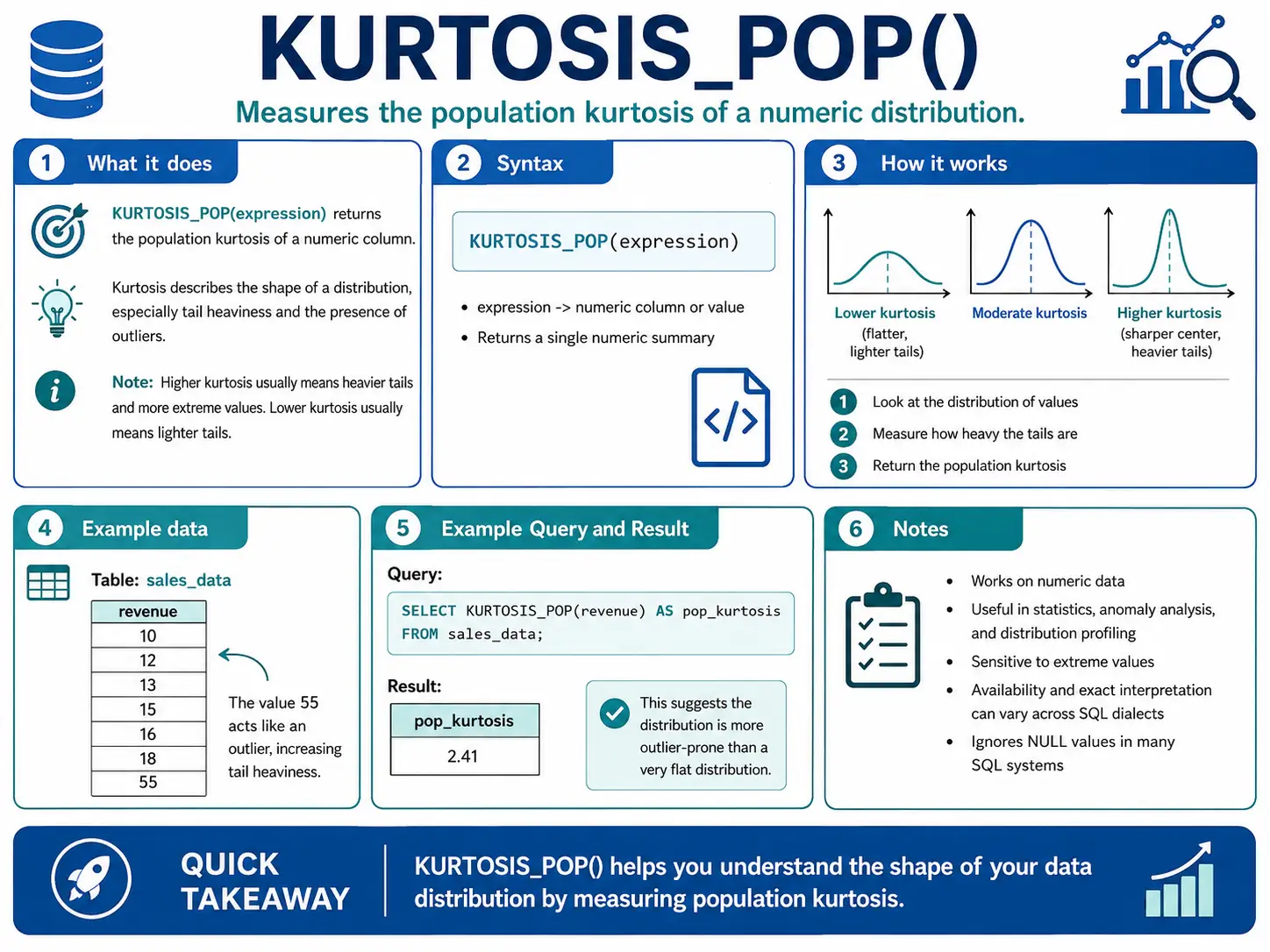
KURTOSIS_POP(): (Oracle) How “Peaky” or “Flat” is My Knowledge?

KURTOSIS_POP() measures the “tailedness” of your knowledge distribution. In easy phrases, it tells you in case your knowledge has only a few excessive values (flat) or many excessive values (peaky). That is necessary for understanding threat or uncommon occasions.

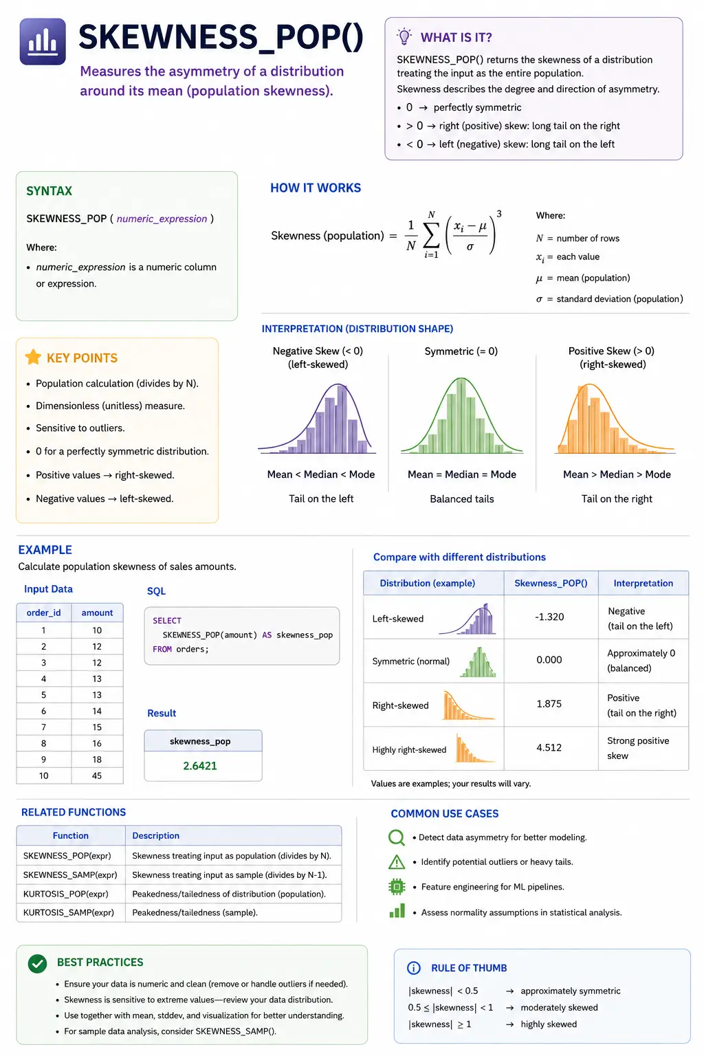
SKEWNESS_POP()

SKEWNESS_POP() measures how symmetrical your knowledge is. In case your knowledge is completely balanced round its common, it has zero skewness. Constructive skew means extra knowledge is on the left (an extended tail to the appropriate), and detrimental skew means extra knowledge is on the appropriate (an extended tail to the left).

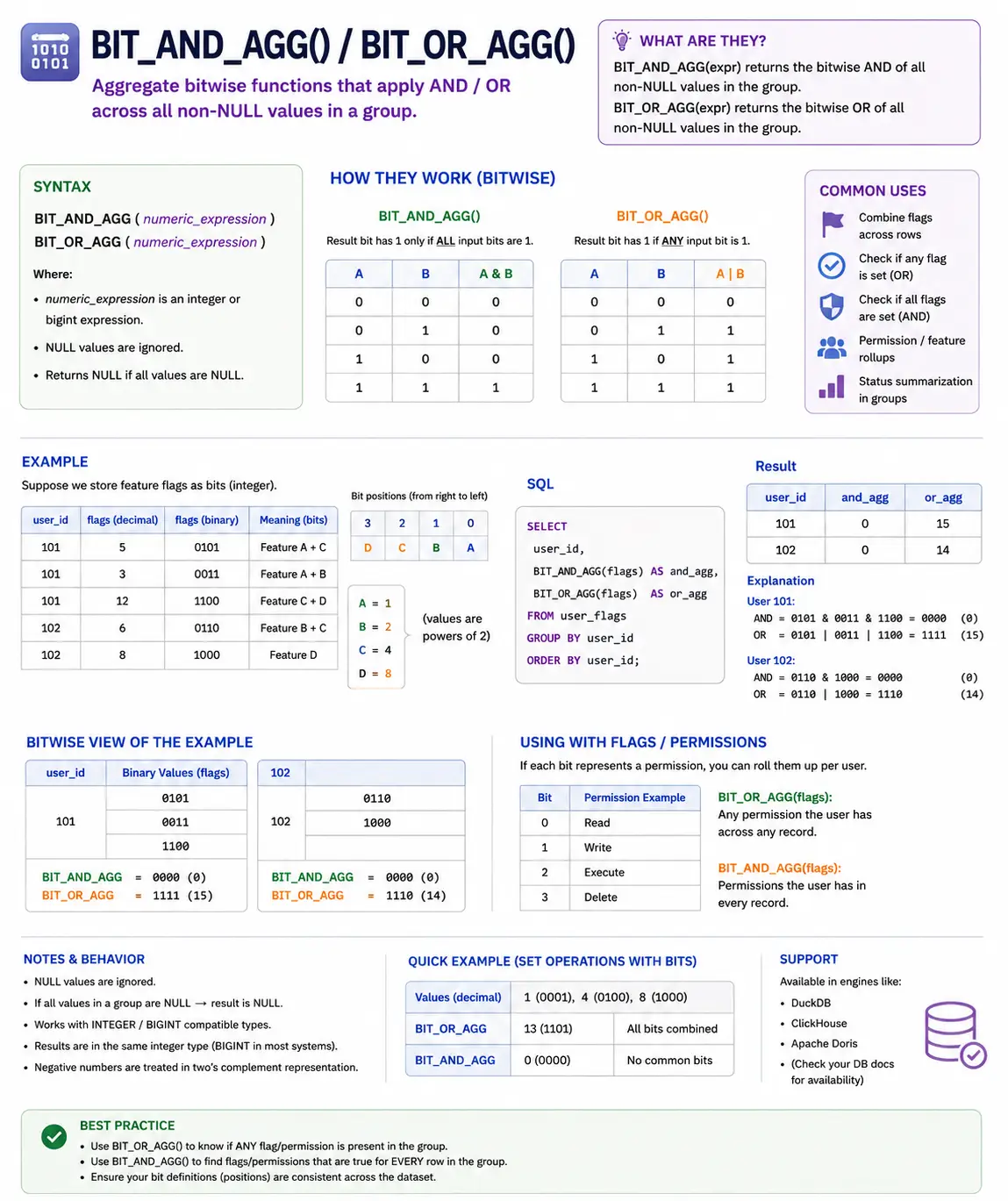
BIT_AND_AGG() / BIT_OR_AGG(): (BigQuery/Oracle) Combining Binary Flags

These are particular features for working with binary numbers (bits). In case you have flags or permissions saved as bits, BIT_AND_AGG() will discover the widespread bits (permissions) throughout a gaggle, and BIT_OR_AGG() will discover all bits (permissions) current in at the least one merchandise within the group.

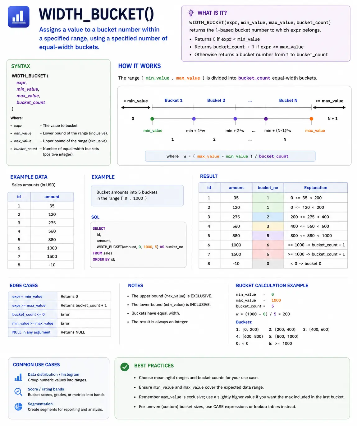
WIDTH_BUCKET(): Grouping Knowledge into Buckets

WIDTH_BUCKET() is a helpful perform for dividing a variety of values right into a specified variety of equally sized buckets or bins. That is nice for creating histograms or categorizing steady knowledge.

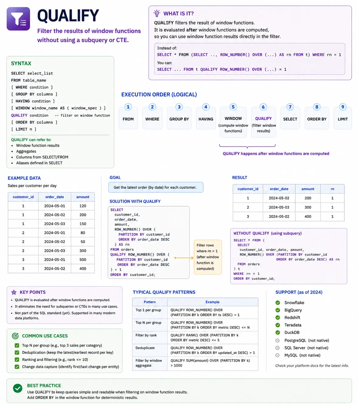
QUALIFY: Filtering Window Operate Outcomes (Snowflake/BigQuery)

QUALIFY will not be a perform itself, however a robust clause obtainable in some fashionable SQL dialects (like Snowflake and BigQuery) that permits you to filter the outcomes of window features straight, without having to wrap your question in a subquery or CTE. It makes your code a lot cleaner whenever you need to choose rows based mostly on a window perform’s output.

Understanding SQL’s Execution Order: When Do WIndow Capabilities Run?

To make use of window features successfully, that you must perceive when SQL truly calculates them. SQL doesn’t learn your question from high to backside. It follows a selected logical order:

1. FROM & JOIN: First, SQL will get the tables and joins them collectively.
2. WHERE: Then, it filters out rows that don’t match your situations.
3. GROUP BY: Subsequent, it teams rows collectively for normal mixture features.
4. HAVING: It filters these grouped rows.
5. SELECT: Now, it picks the columns you requested for. That is the place Window Capabilities are calculated!
6. DISTINCT: It removes duplicate rows.
7. ORDER BY: Lastly, it types the ultimate outcomes.
8. LIMIT / OFFSET: It restricts the variety of rows returned.

Why does this matter? As a result of window features are calculated in step 5 (SELECT), they occur after the WHERE clause. This implies you can not use a window perform straight in a WHERE clause to filter your outcomes.

Conclusion

SQL Window Capabilities are an absolute must-have talent for any knowledge scientist. They let you carry out complicated, row-level calculations with out dropping the element of your unique knowledge. By mastering these 40 features from fundamental rating to superior statistical evaluation you’ll have the ability to write cleaner, extra environment friendly queries and uncover deeper insights out of your datasets.

Continuously Requested Questions